
|
Jupyter at Bryn Mawr College |
|
|
| Public notebooks: /services/public/dblank / CS371 Cognitive Science / 2016-Fall | |||
1. Introduction to Robots
1.1 Introduction to Agent-Based Modeling
CS371: Cognitive Science
Bryn Mawr College
Doug Blank
1.2 Ladybug Robot Simulation
Our first simulation is a discrete simulation: the world is divided into discrete locations (called patches) and the world operates in discrete time steps.
A Ladybug world looks like this:
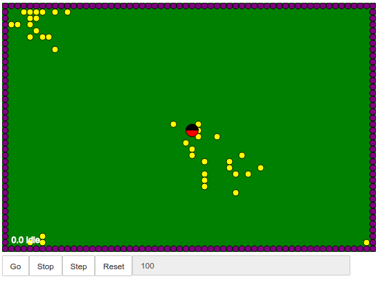
You will be writing a brain for the Ladybug, the black and red circle in the middle of the world. In the above image, ladybug is facing up. Ladybug can:
- turn left or right, but only in a grid-like manner
- go forward or backward specific distances
- sense the world immediately in front of it, and in its peripheral view
1.3 Writing a Brain
Brains for the Ladybug Simulation are composed of a set of rules. You can have as many rules as you wish.
Rules are composed of the following parts, separated by spaces:
STATE SENSE-PATTERN -> ACTION NEXT-STATE
In your brain, you can also have comments (lines that start with a #) and blank lines. Here is a very simple brain:
# This is my first brain!

0         *****          ->    forward(1)  0
Next, let's examine each part of a rule to find out what this does.
1.3.1 STATE and NEXT-STATE
State is a name used as a simple memory for your ladybug. Ladybugs always start out in state "0". States can be any name with no spaces.
1.3.2 SENSE-PATTERN
Ladybugs can see in the 5 cells near the front of its head. In the following pictures, the ladybug can see the patches with a yellow circle in the, and cannot see the patches that are just green.
Facing up:
 |
|
|
|---|---|---|
|
 |
|
 |
|
|
Facing right:
|
|
|
|---|---|---|
|
 |
|
|
|
|
Facing down:
|
|
|
|---|---|---|
|
 |
|
|
|
|
Facing left:
|
|
|
|---|---|---|
|
 |
|
|
|
|
In the simulator, the ladybug is a bit bigger than its nearby cells, so it overlaps just a little, as you can see here:

The 5 sense locations are matched in the same locations ego-centrally located to the ladybug. So they are always listed in this order:
| left side | in front/left | center/forward | in front/right | right side |
When you write a rule, you can either match a patch exactly, or you can use the "wildcard" character *.
f- foodw- wall*- either food, wall, or open space
1.3.3 ACTION
- forward(DISTANCE) - where DISTANCE is between 1 and 9, inclusive
- backward(DISTANCE) - where DISTANCE is between 1 and 9, inclusive
- turnLeft(DEGREE) - where DEGREE is 90 or 180
- turnRight(DEGREE) - where DEGREE is 90 or 180
- stop()
0 ***** -> forward(1) 0
Finally, in order to run your rules in the simulation, we must use a little magic.
%%simulation

# My first brain!

0 ***** -> forward(1) 0
1.4 Putting it all together
Note: ordering is important! Rules are checked for matches from top to bottom.
Your agent has an energy level. It starts at 100, and decreases with the amount of energy it expends. If it gets down to zero, it dies.
Some notes about the world:
- on each restart, the food is randomly placed in the world
- the walls appear as purple circles
%%simulation

# My first brain!

0 ***** -> forward(1) 0
%%simulation

0 **w** -> turnRight(90)  0
0 ***** -> forward(1)     0
1.5 Analysis
Let's analyze the last ladybug's run. We can do a quick plot of the energy over time.
First, we import the simulation library in order to get to the ladybug robot:
from calysto.simulation import get_robot
ladybug = get_robot()
The ladybug keeps track of its energy level at each step in ladybug.history:
str(ladybug.history)
What was the maximum energy level over the run?
max(ladybug.history)
Finally, we can create a quick visualization of the energy level over time:
%matplotlib inline

import matplotlib.pyplot as plt

plt.plot(ladybug.history)
plt.ylabel("Energy")
plt.xlabel("Time")
plt.show()
